Classification

What is Logistic Regression ?

Logistic Regression is a classification algorithm. It is used to predict a binary outcome (1 / 0, Yes / No, True / False) given a set of independent variables. To represent binary / categorical outcome, we use dummy variables. You can also think of logistic regression as a special case of linear regression when the outcome variable is categorical, where we are using log of odds as dependent variable. In simple words, it predicts the probability of occurrence of an event by fitting data to a logit function.

Derivation of Logistic Regression Equation

Logistic Regression is part of a larger class of algorithms known as Generalized Linear Model (glm). In 1972, Nelder and Wedderburn proposed this model with an effort to provide a means of using linear regression to the problems which were not directly suited for application of linear regression. Infact, they proposed a class of different models (linear regression, ANOVA, Poisson Regression etc) which included logistic regression as a special case.

The fundamental equation of generalized linear model is:

g(E(y)) = α + βx1 + γx2

Here, g() is the link function, E(y) is the expectation of target variable and α + βx1 + γx2 is the linear predictor ( α,β,γ to be predicted). The role of link function is to ‘link’ the expectation of y to linear predictor.

Important Points

GLM does not assume a linear relationship between dependent and independent variables. However, it assumes a linear relationship between link function and independent variables in logit model.

1. The dependent variable need not to be normally distributed.
2. It does not uses OLS (Ordinary Least Square) for parameter estimation. Instead, it uses maximum likelihood estimation (MLE).
3. Errors need to be independent but not normally distributed. 

Let’s understand it further using an example:

We are provided a sample of 1000 customers. We need to predict the probability whether a customer will buy (y) a particular magazine or not. As you can see, we’ve a categorical outcome variable, we’ll use logistic regression.

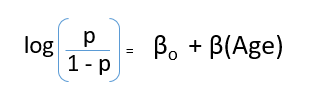
To start with logistic regression, I’ll first write the simple linear regression equation with dependent variable enclosed in a link function:

                           g(y) = βo + β(Age)         ---- (a)

Note: For ease of understanding, I’ve considered ‘Age’ as independent variable.

In logistic regression, we are only concerned about the probability of outcome dependent variable ( success or failure). As described above, g() is the link function. This function is established using two things: Probability of Success(p) and Probability of Failure(1-p). p should meet following criteria:

1. It must always be positive (since p >= 0)
2. It must always be less than equals to 1 (since p <= 1)

Now, we’ll simply satisfy these 2 conditions and get to the core of logistic regression. To establish link function, we’ll denote g() with ‘p’ initially and eventually end up deriving this function.

Since probability must always be positive, we’ll put the linear equation in exponential form. For any value of slope and dependent variable, exponent of this equation will never be negative.

p = exp(βo + β(Age)) = e^(βo + β(Age))    ------- (b)

To make the probability less than 1, we must divide p by a number greater than p. This can simply be done by:

p  =  exp(βo + β(Age)) / exp(βo + β(Age)) + 1   =   e^(βo + β(Age)) / e^(βo + β(Age)) + 1    ----- (c)

Using (a), (b) and (c), we can redefine the probability as:

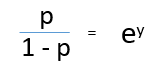
              p = e^y/ 1 + e^y           --- (d)

where p is the probability of success. This (d) is the Logit Function

If p is the probability of success, 1-p will be the probability of failure which can be written as:

q = 1 - p = 1 - (e^y/ 1 + e^y)    --- (e)

where q is the probability of failure

On dividing, (d) / (e), we get,

After taking log on both side, we get,

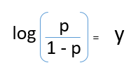
log(p/1-p) is the link function. Logarithmic transformation on the outcome variable allows us to model a non-linear association in a linear way.

After substituting value of y, we’ll get:

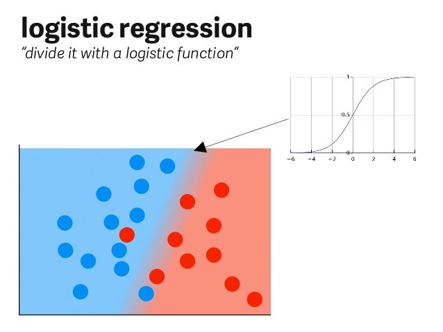
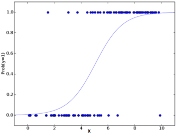
This is the equation used in Logistic Regression. Here (p/1-p) is the odd ratio. Whenever the log of odd ratio is found to be positive, the probability of success is always more than 50%. A typical logistic model plot is shown below. You can see probability never goes below 0 and above 1.